What is an imbalanced dataset?
Most algorithms for machine learning assume that the training set data classes are balanced. But a lot of real world scenarios present classification problems where the involved classes aren’t equally represented: one class is composed by a large number of instances, while the other contains a small number of examples. In this case, the learning algorithm may have difficulties learning the concepts representing the minority class.
Imagine that you are trying to predict the probability that a client leaves your platform (churn analysis). If your product have a good retention ratio, after extracting the dataset from the historical data, your users dataset will contain a lot of examples of people renewing and a minority cancelling their service pack.
Detection of fraudulent transactions, medical diagnosis and detection of oil spills in satellital images are other examples of problems where one of the classes in the dataset is over-represented.
This kind of datasets usually result in the accuracy paradox. Imagine a binary classification algorithm, trying to maximize the predictive accuracy of the model, learning from an imbalanced dataset where 99% of the data is from one class: it could construct a trivial classifier that labels every new case as the majority class, ¡achieving a 99% accuracy! This is especially dangerous when the cost of misclassification of the minority class is high.
Example
I will construct an artificial imbalanced dataset using make_moons, a sklearn
method to generate a dataset with two classes distributed as interleaving half circles.
I also used make_imbalance method from imbalanced-learn library to skew the
dataset and create a majority / minority class with a minority class representing
the 10% percent of the dataset:
import matplotlib.pyplot as plt
import seaborn as sns

from sklearn.datasets import make_moons
from imblearn.datasets import make_imbalance

N_SAMPLES = 1500
MINORITY_RATIO = 0.1

X_balanced, y_balanced = make_moons(n_samples=N_SAMPLES,
                                    shuffle=True,
                                    noise=0.3,
                                    random_state=10)
X, y = make_imbalance(X_balanced,
                      y_balanced,
                      ratio=MINORITY_RATIO,
                      min_c_=1)

f, (ax1, ax2) = plt.subplots(1, 2, sharey=True, sharex=True)

ax1.set_title("Balanced")
ax1.scatter(X_balanced[:, 0], X_balanced[:, 1], marker='o', c=y_balanced)

ax2.set_title("Imbalanced")
ax2.scatter(X[:, 0], X[:, 1], marker='o', c=y)
plt.show()
Measuring the model performance
A classifier in supervised learning is tipically evaluated using a confusion matrix, with columns representing the predicted class and rows representing the actual class. I will use examples of binary classification, but this is generalizable to any number of classes.
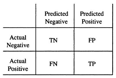
In the confusion matrix, the True Negatives (TN) represent the number of instances of the negative class correctly classified, while False Positives (FP) are the negative instances classified as positive. False Negatives (FN) are those example instances of positive class in the test data that are labeled by the predictor as negative; and True Positives (TP) represent those instances of the positive class correctly classified.
The accuracy score is an evaluation metric that defines the predictive accuracy of the model as (TP + TN) / (TP + FP + TN + FN).
Unfortunately, this accuracy score is not enought to describe the accuracy of a model when confronting imbalanced datasets, or when the cost of misclassification differs between classes.
A good example of this is the Mammography dataset, a skewed data set with a total of 11183 samples with 260 representing calcifications, the positive class. It’s also important to improve the sensity of the positive class in the resultant model, due to the nature of the problem.
To avoid the problems related with accuracy score when dealing with imbalanced data, Area Under the ROC Curve (AUC) has emerged as a popular choice for model performance measurement (Ferri et al, 2004).
Approaches to the problem
The methods proposed to deal with the class imbalance problem could be divided in two main categories: those centered in modifying the learner (algorithm / cost function based) and those centered in balancing the training dataset (resampling based).
The sampling methods are centered in modifying the data distribution through sampling algorithms that create a balanced dataset from our original imbalanced dataset. This allows to the algorithm to improve the precision of the minority class predictions. There are oversampling (expand the examples of the minority class) and undersampling (shrink the majority class, with a possibility of losing data) methods.
Instead, the methods centered in the algorithm modify it to use cost-sensitive methods that take into account the cost of misclassifying the minority class.
Resampling methods in Python: Imbalanced learn
imbalanced-learn is a Python module implementing a lot of those resampling methods. It’s part of the scikit learn contrib projects, and easily integrable with your scikit learn code. Try it, it’s amazing!
Conclusions
Remember, creating models from imbalanced data could be a difficult task. You should use evaluation methods for your models resulting from imbalanced data that take into account those particularities. Select correctly the learning algorithm, and evaluate using resampling methods for the training dataset. Let me know your experiences!
References
- H. He and E. A. Garcia, “Learning from Imbalanced Data”. IEEE Trans. Knowledge and Data Engineering, vol. 21, issue 9, pp. 1263-‐1284, 2009.
- G. Lemaitre and F. Nogueira and C. K. Aridas. “Imbalanced-learn: A Python Toolbox to Tackle the Curse of Imbalanced Datasets in Machine Learning. CoRR, 2016.